The shared model workflow

Use this notebook

Use Notebook 3: Model workflow for this chapter: open it in the book or download the notebook.

Data Science covers regression, classification, regularised linear models, decision trees, support vector machines, and neural networks. These approaches differ in what relationships they can represent, how they are fitted, and how their predictions are interpreted. In scikit-learn, however, they are often used through the same small set of methods: create an estimator, call .fit(), and then call .predict() or .score().

Samples, features, and targets

Each row in X is one sample, such as one participant. Each column is a feature used to describe that sample. y contains the target value the model should learn to predict, with one target aligned to each row in X.

X.shape → samples × features
y.shape → samples

features = ["mean_rt", "accuracy", "age"]  # input columns
X = analysis[features]                       # feature matrix: rows are samples
y = analysis["group"]                       # target aligned with each row

Split before fitting

from sklearn.model_selection import train_test_split

X_train, X_test, y_train, y_test = train_test_split(
    X, y,                         # split features and matching targets together
    test_size=0.2,                # reserve 20 percent for evaluation
    random_state=42,              # make the split repeatable
    stratify=y,                   # preserve class proportions
)

Fit, predict, evaluate

from sklearn.linear_model import LogisticRegression

model = LogisticRegression(max_iter=1000)  # create the estimator
model.fit(X_train, y_train)                # learn from training rows only

predictions = model.predict(X_test)        # predict held-out rows
accuracy = model.score(X_test, y_test)     # compare predictions with targets

Read the API:

• LogisticRegression(...) creates an object.

• .fit(...) is a method that learns from training data.

• .predict(...) is a method that returns predictions.

• .coef_ is an attribute created during fitting.

Pipelines prevent leakage

Common mistake

Calling fit_transform() on the complete dataset before splitting lets test rows influence learned preprocessing values. Split first, then fit the pipeline on the training rows only.

Preprocessing steps learn from data too. For example, StandardScaler calculates a mean and standard deviation for every feature. If it sees the full dataset before the train/test split, information from the test rows has already influenced the training process. This is data leakage: the evaluation is no longer based on completely unseen data.

A pipeline keeps the operations together. When the pipeline is fitted on X_train, the scaler estimates its parameters from X_train only and passes the transformed values to the classifier. Calling .predict(X_test) then applies those stored training parameters to the test rows.

from sklearn.pipeline import make_pipeline
from sklearn.preprocessing import StandardScaler

model = make_pipeline(
    StandardScaler(),                       # fit scaling inside the pipeline
    LogisticRegression(max_iter=1000),      # fit the classifier second
)

model.fit(X_train, y_train)                 # learns all parameters from training data

The scaler is fitted only using training data.

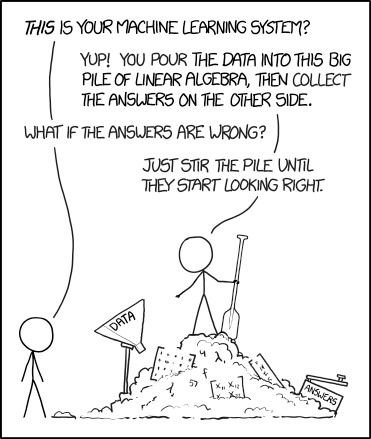
Fig. 7 The interface may be short, but the fitted model still needs to be tested and interpreted. “Machine Learning” by Randall Munroe, licensed CC BY-NC 2.5.

Exercise 20 (Leakage check)

What is wrong with scaling the complete dataset before train_test_split?

Hint

Ask which rows contribute to the means and standard deviations learned by the scaler. Should test rows influence any quantity used during training?

Solution to Exercise 20 (Leakage check)

Information from the test set influences the scaling parameters. The test set is no longer fully unseen. Put scaling inside a pipeline fitted on training data.

Reproducibility

Use explicit random seeds when randomness is part of the computation:

rng = np.random.default_rng(42)
train_test_split(..., random_state=42)

A seed does not make a flawed analysis valid; it makes the same analysis repeatable.

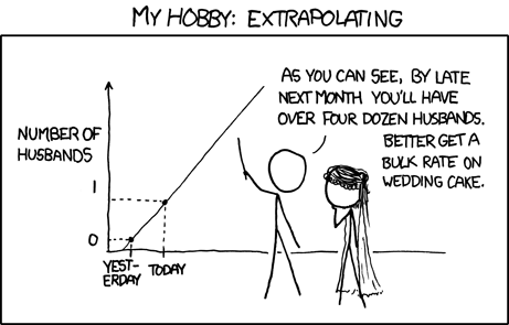
Fig. 8 A model can behave sensibly on held-out observations from the same setting and still fail when asked to predict far beyond them. “Extrapolating” by Randall Munroe, licensed CC BY-NC 2.5.